Specifying Your Own Distribution • distionary

library(distionary)

This vignette explains how to create user-defined distributions using distionary.

User-Defined Distributions

You can make your own distribution using the distribution() function. Specify distribution properties as name-value pairs, where the name is the distribution property. Distributional representations like the cumulative distribution function (CDF) can be specified as functions.

my_normal <- distribution(
  density = stats::dnorm,
  cdf = stats::pnorm,
  range = c(-Inf, Inf),
  g = 9.81,
  another_representation = function(x) x^2,
  .vtype = "continuous"
)
# Inspect
my_normal
#> Unnamed distribution (continuous) 
#> --Parameters--
#> NULL

The usual evaluation framework can now be accessed, such as evaluating the CDF.

eval_cdf(my_normal, at = c(0.2, 0.5, 0.7))
#> [1] 0.5792597 0.6914625 0.7580363

Even though the mean has not been specified, it can still be evaluated.

mean(my_normal)
#> [1] 0

Some of the specified properties are special because they correspond to a property that’s known to distionary – in this example, density, cdf, and range. In general, the special names can be identified as follows:

The suffix following eval_ for any distributional representation (e.g., quantile for eval_quantile()). These should be specified as functions.
realise or realize, which is used to generate random samples from the distribution. This should be a function of the number of observations to draw.
The same name as the distionary functions used to extract any other property (e.g., mean for mean()).

See the Evaluate a Distribution vignette for more details on these evaluation functions and the network of relationships between the understood properties. Note that, in the current version, specifying a cdf along with a density or pmf (probability mass function) is required for evaluating non-explicit properties.

In general, properties can be invoked by the more general function eval_property(), which is useful for accessing entries that are not known to distionary. For example, the user-defined property g can be accessed in this way.

eval_property(my_normal, "g")
#> [1] 9.81

To use eval_property() to evaluate a function, arguments can be specified in the ... argument.

eval_property(my_normal, "another_representation", 1:4)
#> [1]  1  4  9 16

The eval_property() function is also useful for programmatically accessing distribution properties.

properties <- c("mean", "variance")
lapply(properties, \(x) eval_property(my_normal, x))
#> [[1]]
#> [1] 0
#> 
#> [[2]]
#> [1] 1

Distribution Attributes

Distribution metadata are stored as attributes, and are those arguments prefixed by . in the distribution() function.

.vtype, as seen in the example starting this vignette, is used to specify the variable type, such as "discrete" or "continuous".
.name allows you to give the distribution a name.
.parameters allows you to specify values for the distribution’s parameters as a list, if applicable. This version of distionary does not draw from these values, so it currently serves a similar function as the distribution’s name.

my_distribution <- distribution(
  cdf = pnorm,
  density = dnorm,
  .vtype = "continuous",
  .name = "Special",
  .parameters = list(theta = 1.7, mat = diag(2), hello = "hi")
)
# Inspect
my_distribution
#> Special distribution (continuous) 
#> --Parameters--
#> $theta
#> [1] 1.7
#> 
#> $mat
#>      [,1] [,2]
#> [1,]    1    0
#> [2,]    0    1
#> 
#> $hello
#> [1] "hi"

Retrieve the variable type:

vtype(my_distribution)
#> [1] "continuous"

Retrieve the parameters:

parameters(my_distribution)
#> $theta
#> [1] 1.7
#> 
#> $mat
#>      [,1] [,2]
#> [1,]    1    0
#> [2,]    0    1
#> 
#> $hello
#> [1] "hi"

You can also reset the parameters with <-. Lets give this distribution scalar parameters.

parameters(my_distribution)[["mat"]] <- 1
parameters(my_distribution)[["hello"]] <- NULL
# Inspect the distribution
my_distribution
#> Special distribution (continuous) 
#> --Parameters--
#> theta   mat 
#>   1.7   1.0

Retrieve the distribution’s name with pretty_name().

pretty_name(my_distribution)
#> [1] "Special"

Names are “pretty” because they can also include the parameters in a compact way, when the parameters are scalars (which they now are):

pretty_name(my_distribution, param_digits = 2)
#> [1] "Special(1.7, 1)"

Example of a New Parametric Family

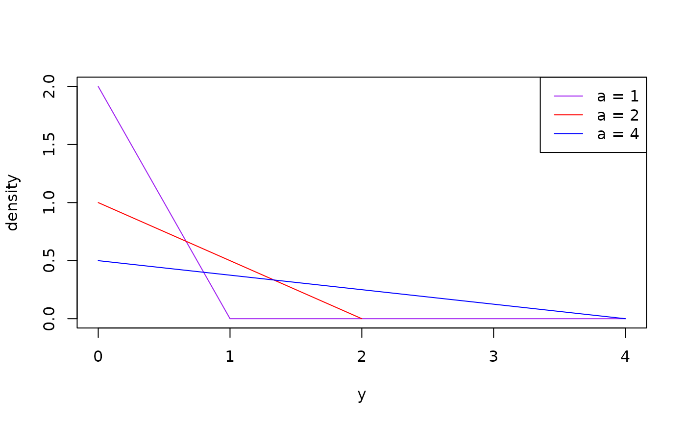
If you want to create your own parametric family, such as a distribution whose density decays linearly from x=0 to x=a, you can do this by making a function that accepts the distribution parameter as an input, and outputs the distribution. Note that the CDF and density are specified, as required for continuous distributions, and metadata are specified with the arguments starting with ..

dst_linear <- function(a) {
  # It helps to check that the parameter is valid.
  checkmate::assert_number(a, lower = 0)
  # We'll create some representations outside of the `distribution()`
  # call for separation of concerns. Note that care is taken to ensure
  # proper behaviour outside of the range of the distribution.
  density <- function(x) {
    d <- 2 / a^2 * (a - x)
    d[x < 0 | x > a] <- 0
    d
  }
  cdf <- function(x) {
    p <- x / a^2 * (2 * a - x)
    p[x < 0] <- 0
    p[x > a] <- 1
    p
  }
  # Create the distribution.
  distribution(
    density = density,
    cdf = cdf,
    range = c(0, a),
    .vtype = "continuous",
    .name = "Linear",
    .parameters = list(a = a)
  )
}

Notice how the distribution metadata gets printed with the distribution.

dst_linear(3)
#> Linear distribution (continuous) 
#> --Parameters--
#> a 
#> 3

Here are the density plots of different members of this family.

plot(dst_linear(1), to = 4, col = "purple")
plot(dst_linear(2), add = TRUE, col = "red")
plot(dst_linear(4), add = TRUE, col = "blue")
legend(
  "topright",
  legend = c("a = 1", "a = 2", "a = 4"),
  col = c("purple", "red", "blue"),
  lty = 1
)

As usual, properties can be evaluated, even if they are not specified. Consider, for example, calculating return periods of three different Linear distributions.

enframe_return(
  model1 = dst_linear(1),
  model2 = dst_linear(2),
  model3 = dst_linear(4),
  at = c(2, 5, 10, 20, 50, 100),
  arg_name = "return_period"
)
#> # A tibble: 6 × 4
#>   return_period return_model1 return_model2 return_model3
#>           <dbl>         <dbl>         <dbl>         <dbl>
#> 1             2         0.293         0.586          1.17
#> 2             5         0.553         1.11           2.21
#> 3            10         0.684         1.37           2.74
#> 4            20         0.776         1.55           3.11
#> 5            50         0.859         1.72           3.43
#> 6           100         0.900         1.80           3.60

Network of Properties

The key innovation in distionary is its network-based approach to probability distributions. Different distributional representations (CDF, PDF/PMF, quantile function, survival function, etc.) are interconnected through a network of mathematical relationships.

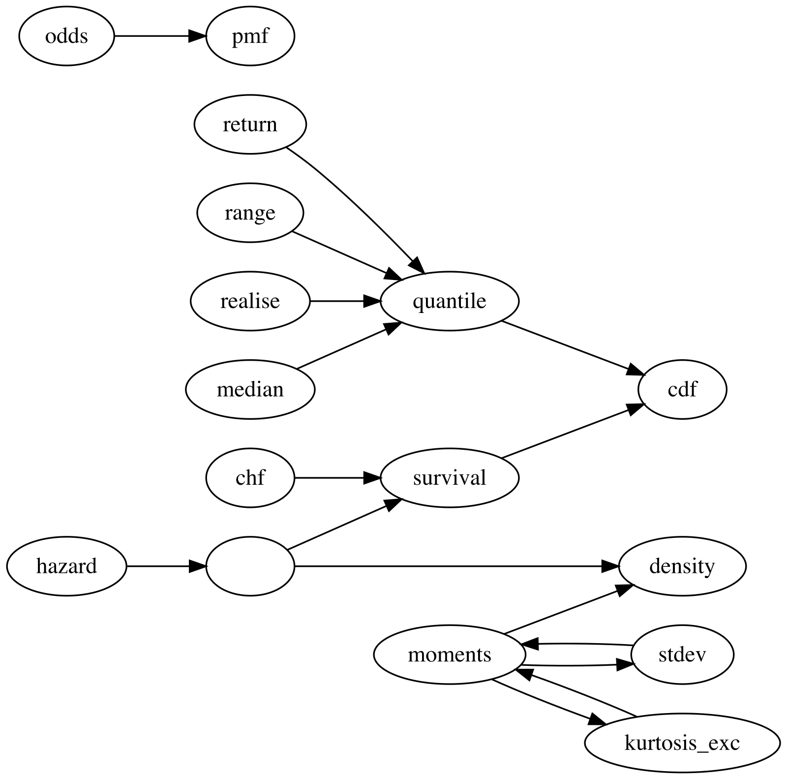
The diagram below shows how distionary derives distribution properties from other properties. An arrow from one property to another indicates that the first property can be calculated from the second. For example, quantile can be calculated from cdf, and mean can be calculated from density. This network structure is what allows you to define a custom distribution with just one or two representations (like cdf and density in the example above) and still have access to all other properties.

Making your own properties

Some properties are easy to make yourself. Here is an example of a function that calculates interquartile range.

# Make a function that takes a distribution as input, and returns the
# interquartile range.
iqr <- function(distribution) {
  diff(eval_quantile(distribution, at = c(0.25, 0.75)))
}

Apply the function to a Linear distribution as defined before.

iqr(dst_linear(2))
#> [1] 0.7320508

For properties that are not handled by distionary (e.g., extreme value index, or moment generating function), one option is to build these properties into your own distribution. A future version of distionary will make user-defined properties easier to work with.

Limitations

The distionary package is still young. Lots of helpful features are still missing, and your patience is appreciated as more features are developed. Some examples follow.

#	Limitation	Explanation
1.	When a user-specified distribution isn’t continuous (e.g., is discrete), only the properties specified in `distribution()` can be accessed in this version.	Specifying the set of possible outcomes for discrete distributions requires special attention, particularly when there are infinitely many of them.
2.	Representations are not checked for accuracy in this version.	While this is done in the test suite for the built-in distributions, additional levels of detail are required when accepting a foreign distribution.
3.	Typos when specifying distribution property names (e.g. `densty` instead of `density`) or variable type (e.g., `"contnous"` instead of `"continuous"`) will not trigger an error.	The package does not assume that distribution properties and types are limited, allowing for flexibility.
4.	It is currently assumed that the distributional representations are specified in a way that remains valid beyond the range of the distribution.	A future version aims to use the specified range to automatically implement appropriate behavior.