Built-In Distributions • distionary

library(distionary)

This vignette covers built-in distribution families available in distionary. It provides insight into each family and its counterparts in the stats package.

Built-In Distribution Families

All distribution families found in the stats package are integrated into distionary, along with a few others. They are shown in the table below with notes on whether they have counterparts in the stats package.

Distribution	`distionary` Function	Has counterpart in `stats`
Bernoulli	`dst_bern()`	Yes
Beta	`dst_beta()`	Yes
Binomial	`dst_binom()`	Yes
Cauchy	`dst_cauchy()`	Yes
Chi Squared	`dst_chisq()`	Yes
Degenerate	`dst_degenerate()`	No
Exponential	`dst_exp()`	Yes
Empirical	`dst_empirical()`	No
F	`dst_f()`	Yes
Finite	`dst_finite()`	No
Gamma	`dst_gamma()`	Yes
Geometric	`dst_geom()`	Yes
Generalised Extreme Value (GEV)	`dst_gev()`	No
Generalised Pareto (GP)	`dst_gp()`	No
Hypergeometric	`dst_hyper()`	Yes
Log Normal	`dst_lnorm()`	Yes
Log Pearson Type III	`dst_lp3()`	No
Negative Binomial	`dst_nbinom()`	Yes
Normal	`dst_norm()`	Yes
Pearson Type III	`dst_pearson3()`	No
Poisson	`dst_pois()`	Yes
Student t	`dst_t()`	Yes
Uniform	`dst_unif()`	Yes
Weibull	`dst_weibull()`	Yes

In addition, there is a special “Null” distribution object akin to a missing or unknown distribution. This is useful, for example, if an algorithm fails to return a distribution: instead of throwing an error, a Null distribution can be returned.

# Make a Null distribution.
null <- dst_null()
# Inspect
null
#> Null distribution (NA)

This is the behaviour when specifying NA as a distribution parameter:

dst_norm(mean = 0, sd = NA)
#> Null distribution (NA)

The Null distribution always evaluates to NA.

mean(null)
#> [1] NA
eval_pmf(null, at = 1:10)
#>  [1] NA NA NA NA NA NA NA NA NA NA
range(null)
#> [1] NA NA

The Empirical Distribution

The Empirical distribution is different from the others in terms of its utility because it makes your data the distribution, and is therefore far more flexible than any of the other distributions.

In statistical terminology, this is because the other built-in distributions are parametric, defined by a fixed amount of numeric parameters. For example, exactly two parameters make up the family of Normal distributions. The empirical distribution, on the other hand, is a non-parametric model, because there isn’t a fixed number of numeric parameters that can describe it.

The Empirical distribution is particularly advantageous when a distribution’s standard form is unknown or infeasible to model, or when comparing a custom model against data is needed.

Here is an example of forming an empirical distribution from a dataset generated from a Normal distribution. First, define the normal distribution and generate a sample; the first few observations are shown below.

set.seed(42)
normal <- dst_norm(0, 1)
x <- realise(normal, n = 100)
# Inspect the first few observations
head(x)
#> [1]  1.3709584 -0.5646982  0.3631284  0.6328626  0.4042683 -0.1061245

An Empirical distribution can be made from these values.

empirical <- dst_empirical(x)
# Inspect
empirical
#> Finite distribution (discrete) 
#> --Parameters--
#> # A tibble: 100 × 2
#>    outcomes probs
#>       <dbl> <dbl>
#>  1    -2.99  0.01
#>  2    -2.66  0.01
#>  3    -2.44  0.01
#>  4    -2.41  0.01
#>  5    -1.78  0.01
#>  6    -1.76  0.01
#>  7    -1.72  0.01
#>  8    -1.46  0.01
#>  9    -1.39  0.01
#> 10    -1.37  0.01
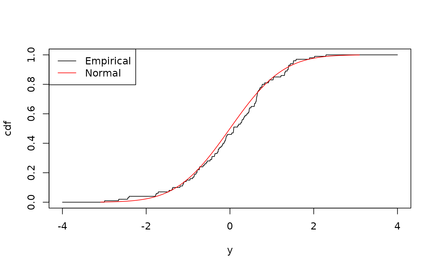
#> # ℹ 90 more rows

Comparing its CDF to the normal distribution, one can see the two are similar:

plot(empirical, "cdf", from = -4, to = 4, n = 1000)
plot(normal, "cdf", add = TRUE, col = "red")
legend(
  "topleft", 
  legend = c("Empirical", "Normal"), 
  col = c("black", "red"), 
  lty = 1
)

Although this distribution is non-parametric, the parameters() function is still applicable because it’s not tied to the statistical definition of “parametric”, which is concerned with parameter dimension. In distionary, the dataset itself and their probabilities comprise the distribution parameters (using str() here for better printing):

str(parameters(empirical))
#> List of 2
#>  $ outcomes: num [1:100] -2.99 -2.66 -2.44 -2.41 -1.78 ...
#>  $ probs   : num [1:100] 0.01 0.01 0.01 0.01 0.01 0.01 0.01 0.01 0.01 0.01 ...

One should also note that Empirical distributions are discrete, with outcomes defined by the observed values:

vtype(empirical)
#> [1] "discrete"